Hey everyone! I have recently been working on various ways to improve the lighting on niagara particles. I will use this thread as a repository for multiple techniques I have been messing with.
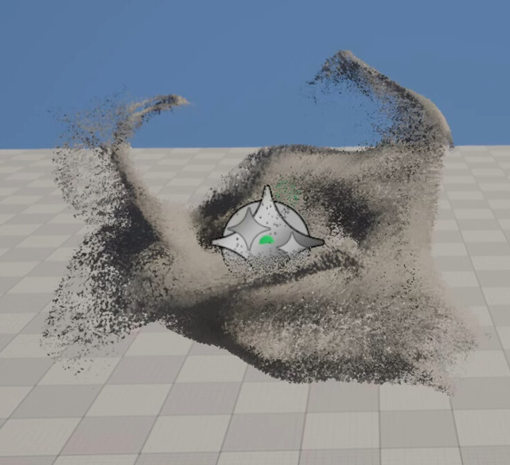
This is the most recent technique I have been working on. I wanted to achieve particle normals based on a density gradient. I am using the neighbor grid 3d to save the particle counts in each cell and then I do a gradient calculation along each axis. The final vector is fed into the materials via the dynamic materials parameter and plugged into the normals slot. I can also control the delta offset for the gradient calculation, the larger the offset, the smoother/more blurred the resulting normals become. Smaller values will capture more high frequency details but can become noisy if you go too low. Enjoy, Feedback welcome!
That’s a really fun idea.
Care to share some more information?
How many grid cells do you need to get the quality you want? I imagine there’s some tradeoff where more cells give you more accurate gradients, but less information about the nearby particles.
What’s the cost of running this right now? Did you do any profiling?
I can get the cost down as low as 0.1ms with a 64x64x64 grid and 500k particles which gives decent results. There is diminishing returns the more dense you make the grid. There is a weird quirk where i can actually get good results with a grid of 1x1x1 and a neighbor count of 999,999,999. Oddly, in some situations, having a higher neighbor count actually reduces cost, sometimes dramatically. There seems to be a relationship between the max particle per cell and the cell count. Not sure exactly what black magic is going on, but works…
I am also doing a 3x3x3 sobel sample for each axis and combining the results for the final vector. That is 18 samples per axis, 9 positive and 9 negative. It dramatically smoothed out the results and the extra perf cost wasn’t very bad.
Naturally, if the particles drift outside the grid they wont receive any lighting into and will turn black. I use a kill volume to destroy any particles that leave the grid. If you set this up with local space, dont apply any rotations to the grid or else it will rotate the lighting results too, only do position updates.
Here is the scratchpad version. There are actually several different methods to implement this. depends on what stage you do the offsets for the particles, on the particle locations or the grid cells. I have since moved it into HLSL but im not sure if i will share it yet or not. Copy/paste this text into a new scratchpad in the particle update section and it should make all the nodes. Create a material with a dynamic material param and use an append many to combine the 3 axis. Then transform the normals from world to tangent before plugging into the normals slot in the material. Dont forget to set the offset value in the scratchpad or else it wont work. 2.5 is a good starting point. Lower numbers give you more high frequency detail but it can become very noisy.
You will have to setup the neighbor grid yourself, there are a bunch of videos demonstrating the process. Let me know if you have any questions on getting this working.
This technique seems to work best with many small particles. Its fun to play with but probably a bit impractical for a production setting.
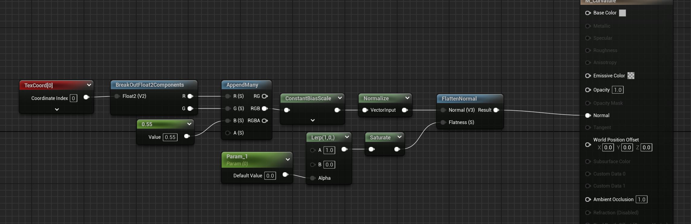
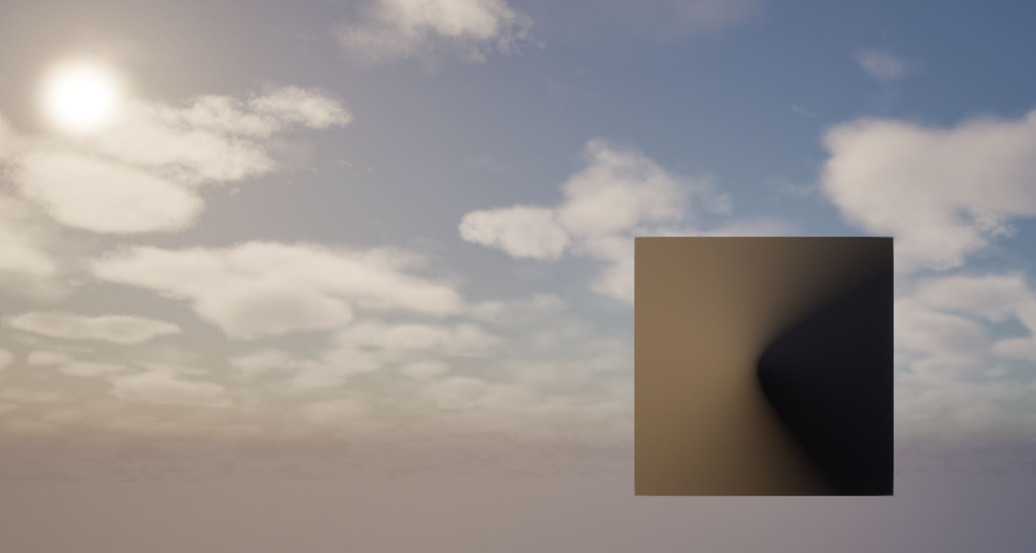
Here is a small setup for a curvature map to give your particles a bit more volume with their lighting. This is my version of epics “generate spherical normals” flag in the particle editor. As I’m sure most of you are aware, that flag isnt very useful because it makes a perfect spherical normal over your sprite and has a really hard edge. If your texture goes outside that spherical normal you will see this edge.
This version isnt exactly a perfect spherical normal, but it will give you a nice gradient across the surface. Its purpose is for particles that are very soft, where an actual normal map might give too much definition, such as soft smoke plumes.
You can adjust the pinch in the center of the normals by adjusting the value being fed into the blue channel (z axis) of the normals. Use values from 0.5-1. 0.5 will make the point in the middle be very sharp, like a normal of a cone, 1 will make it more round like a sphere. The constant bias scale is set to -0.5 and 2. The flatten normal will allow you to adjust how strong this gradient is.